Introduction

Fine-tuning is a crucial step in the development and improvement of artificial intelligence. It involves adapting a pre-trained model to better suit specific tasks or datasets, thereby enhancing its accuracy, efficiency, and overall performance. This process is especially useful when applying models across various industries, where specific requirements can significantly differ. During fine-tuning, the model undergoes additional training on data relevant to the target application. This ensures the model recognizes general patterns and the specific characteristics important for the task. In this way, fine-tuning allows customization of models for diverse use cases, from medical diagnostics to personalized product recommendations.

OpenAI’s CLIP (Contrastive Language-Image Pretraining) model is a prime example of a powerful AI tool, renowned for its ability to understand and relate textual descriptions to images. Fashion CLIP is a fine-tuned version of CLIP, specifically adapted to cater to the needs of the fashion industry and is publicly available on Hugging Face.

We conducted fine-tuning on the Fashion CLIP model to improve its performance in scenarios where it did not initially perform well. Our goal was to adapt it to the specific challenges and tasks of the fashion industry, enabling it to better understand and connect visual and textual data in this context. Specifically, we fine-tuned the model for recognizing and categorizing shoelace colors, addressing a detailed yet important aspect of fashion product identification.

Fashion CLIP

Fashion CLIP, as mentioned before, is a fine-tuned edition of CLIP model. It embeds images and descriptions of various concepts that the original CLIP model was trained on, in addition to fashion concepts. This means that a singular dense vector will represent each image and description, and they are placed in the same vector space for easy comparison.

Both FashionCLIP and CLIP are based on contrastive learning techniques. This represents a machine learning technique that trains a model to differentiate between similar and dissimilar examples by optimizing a Contrastive Loss function. The model consists of a text encoder and an image encoder which vectorizes text and image inputs. The training aims to adjust weights of the two encoders so that similar pairs are close to each other in vector space with reference to cosine similarity, and dissimilar pairs are far from each other. Although there are many different loss functions, while fine-tuning Fashion CLIP it was decided that Contrastive Loss function should be used because CLIP was previously trained and fine-tuned with it.

The dataset

One of the most important things when fine-tuning a model is to choose the right dataset. The dataset needs to closely match the domain and tasks the model will encounter in real-world applications, ensuring that model learns features and patterns that are applicable and useful for its intended use. Diversity of dataset is also important, it helps model to generalize across various scenarios and reduces the risk of overfitting. Sufficient dataset size ensures the model has enough examples to learn robust and generalizable patterns. Too small dataset may lead to overfitting, while too large dataset may include more noise and more irrelevant data.

In summary, the right dataset ensures the model learns relevant, high-quality, diverse, and representative patterns, leading to better performance and generalization when fine-tuning. While choosing our dataset, the main motivation was to use descriptions for the images which would contain information about the shoelace color. This would enable the model to accurately identify and differentiate shoelace colors within the broader context of footwear images.

The Fashion Product Images Dataset from Kaggle was chosen, which contains 44,441 diverse clothing images. From this dataset, we selected only footwear, totaling around 7,344 items.

During model development, it is also important to split the dataset into three subsets: training, testing, and validation. This split helps us assess how well the model learns to recognize new, unseen data. Following recommendations, the dataset was initially split evenly by categories into 80% for training (5,877 images) and 20% for testing (1,467 images). Later, during the testing phase, a validation dataset was created by taking a 10% sample, split evenly by categories, from the training dataset.

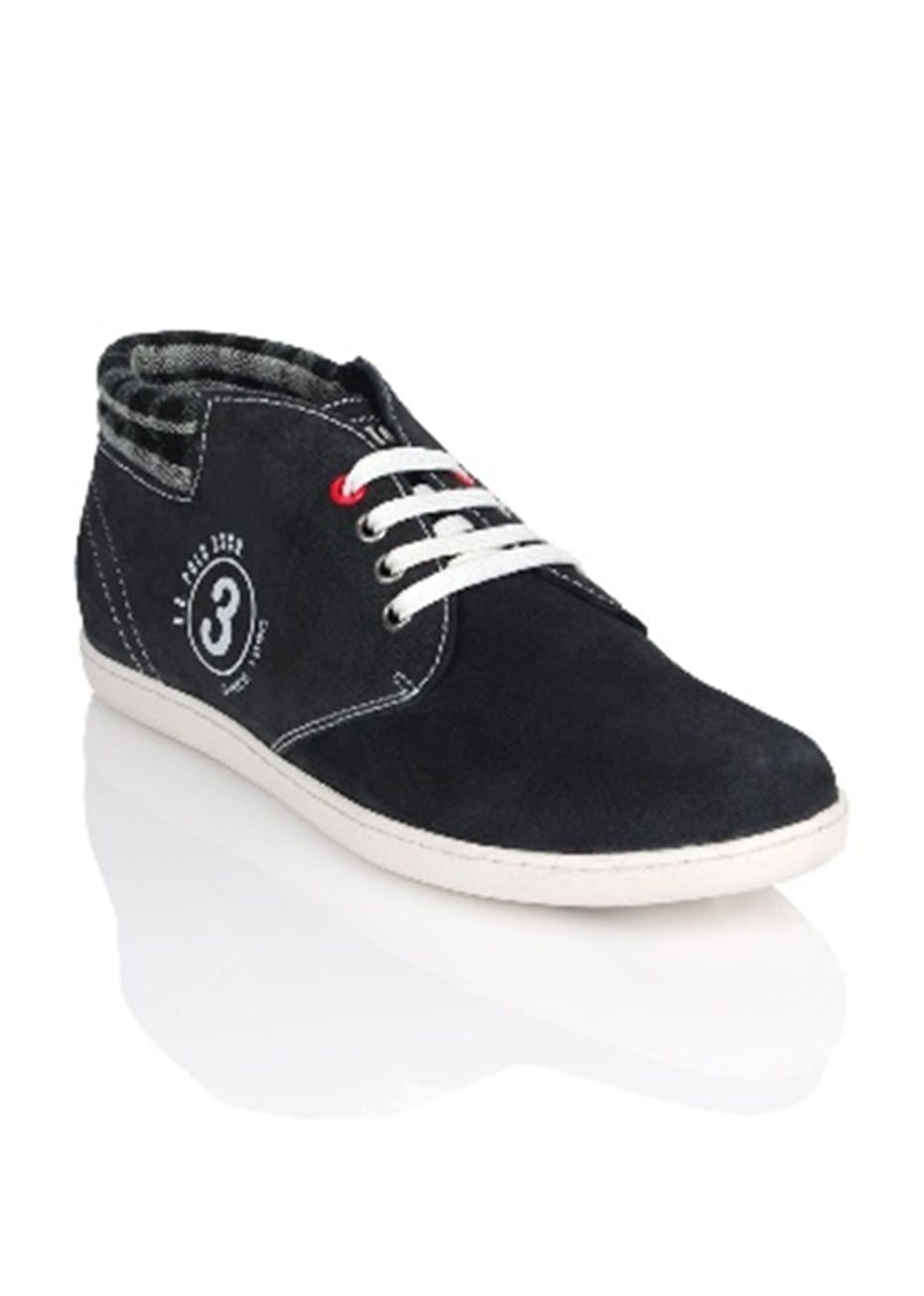
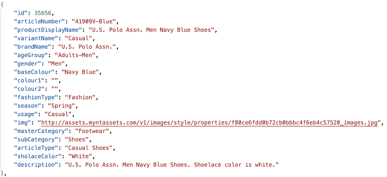
Each item came with its own Json file which consisted of well over 30 fields with a lot of nested items describing it. Files were later adjusted in a way that only 19 fields of significance were used, and they were put all together in one Json file. Out of those 19, one was the image URL, and one was added manually in the last stage of dataset preparation. The example of the item can be seen bellow:

Originally, the dataset included basic descriptions (brand, product name, gender, and main color), but we needed more detailed annotations. We used Bakllava AI tool to enrich the descriptions with the prompt, “Describe the item in the image.” While the generated descriptions varied in detail, they often lacked shoelace color information, so the process of checking and adding correct color to each footwear item was done by hand.

The final dataset fields used to train the model were the image and the enriched description. This description included the original details, an additional sentence from Bakllava AI, and a sentence describing the shoelace color.

Fine-tuning techniques

We used PyTorch Lightning and Google Colab to fine-tune the FashionClip model. We wrote and executed Python code in Jupyter Notebooks directly in the browser. This way, we avoided setting up local machines and leveraged more powerful cloud-based machines.

What is an epoch?

The first thing that needs to be understood when we want to start with fine-tuning is “epoch” and why it is important.

An epoch is one full pass through your entire training and validation dataset. Like flipping through a book’s pages to get the complete picture. During each epoch, the model can see the complete dataset and update its parameters based on what it learns.

In real-world scenarios, data is rarely perfect or covers all possible edge cases by letting the model go through the entire dataset multiple times, it can learn patterns and details. This repetition helps the model generalize better and perform effectively on new data.

Imagine you’re training a model to recognize different types of shoes. In the first epoch, it might learn basic shapes and colors. As it goes through more epochs, it will start noticing finer details like fabric texture or lace designs, improving its ability to recognize shoes accurately.

Batches and their role in training

To make training manageable, especially with large datasets, we split the data into smaller, more digestible chunks called batches. The model processes these batches one at a time.

The size of each batch depends on factors like your dataset’s size and your computational power. For example, if you have 1,000 samples and set a batch size of 100, the model will process the data in 10 steps per epoch.

Breaking the data into batches makes computations more efficient and helps stabilize the training process. Each batch allows the model to make small adjustments, contributing to its overall learning and performance.

The importance of multiple epochs

Training a model effectively often requires multiple passes through the dataset. Each epoch lets the model refine its learning. Early epochs help the model grasp general patterns, while later epochs fine-tune its understanding.

For instance, if you’re training a shoe recognition model for 20 epochs, the model will see each shoe image 20 times throughout the training process. Each pass might shuffle the data, helping the model learn more robust features and reducing the chance of memorizing the data order.

Finding the right number of epochs is a balancing act:

Underfitting: If you train for too few epochs, the model might not learn enough from the data, leading to underfitting, where it performs poorly on both training and new data.

Overfitting: Conversely, if you train for too many epochs, the model might become too tailored to the training data, which is known as overfitting. This means it might not perform well on new data.

To find the right balance, you should monitor the model’s performance on a validation set after each epoch. If the performance on the validation set starts to drop while it’s still improving on the training set, it might be time to stop training to avoid overfitting.

DataLoader Usage

The quality of your dataset is crucial. However, how you handle and process this data can significantly impact your model’s performance. DataLoader manages datasets efficiently. The Dataset class in PyTorch typically includes several functions that facilitate data handling. These functions ensure that data is processed correctly and efficiently, which is essential for model performance. Some of the functions are loading data pairs, configuring DataLoader for our specific needs. When DataLoader is configured then we fetch each item from the provided dataset and ensure that all images and text are ready for model training.

We use DataLoader for loading data in batches for both training and evaluation. It provides several functionalities that make data handling more efficient and effective.

Batching: Batching helps speed up the training process and enables the handling of larger datasets that may not fit into memory if processed individually.

Shuffling: Shuffling randomizes the order of data samples before batching them. This ensures that the model does not learn any unintended patterns from the order in which data is presented.

Parallel Data Loading: DataLoader uses multiple workers to load data in parallel. This means that data loading can occur simultaneously across multiple CPU cores, significantly reducing the time required to prepare data for each batch.

Understanding Optimizers

Optimizers play a crucial role in the training. In our journey to optimize our model, we experimented with various optimizers, including SGD, AdamW, and RMSprop. While SGD showed promise in some scenarios, it required careful tuning of the learning rate and momentum and often struggled with stability due to the smaller dataset size. RMSprop helped make training more stable but produced inconsistent results due to its overly aggressive changes in the learning rate.

Choosing the right optimizer depends on the specific characteristics of the task and the size and complexity of the dataset. Ultimately, we chose AdamW (Adam with weight decay) as our optimizer. AdamW separates weight decay from the gradient update process, allowing for better regularization and control over learning rates. This feature was particularly beneficial given our smaller dataset, helping to prevent overfitting and enhancing generalization.

Configuring Optimizers

Proper configuration of the optimizer is critical for achieving balanced training. Key parameters for AdamW include the:

learning rate – which determines the step size for weight updates

betas – which control the moving averages of the gradient and its square

eps – a small constant for numerical stability

weight decay – which adds a regularization term to the loss function to penalize large weights

Here’s the final configuration for AdamW in our use case:

				
					torch.optim.AdamW(model.parameters(), lr=3e-5, weight_decay=1e-4)

Understanding Schedulers

Schedulers adjust the learning rate during training based on model performance. They play a vital role in fine-tuning the training process. We experimented with different schedulers to find the best fit for our model, including CyclicLR and CosineAnnealingLR. CyclicLR varied the learning rate within a specified range, cycling between a lower and an upper bound. It can be beneficial for training on large datasets where exploration is needed, but it is less suitable for fine-tuning with smaller datasets. CosineAnnealingLR caused the learning rate to vary in a wave-like pattern, which wasn’t suitable for our goal of achieving stable training.

In the end, we decided that ReduceLROnPlateau emerged as the most effective for our smaller dataset. It showed the ability to reduce the learning rate when validation performance stops improving and maintaining a steady training process, proved to be the best choice.

Configuring Schedulers

Key parameters for configuring the ReduceLROnPlateau scheduler include:

mode – specifies whether to monitor the minimum or maximum of the metric

factor – which determines the reduction rate

patience – indicating the number of epochs to wait before reducing the learning rate

threshold – which defines the minimum change to consider an improvement

Our final configuration for the scheduler was as follows:

				
					torch.optim.lr_scheduler.ReduceLROnPlateau(optimizer, mode='min', patience=1, factor=0.1)

This setup ensured that the learning rate was reduced by a factor of 0.1 after two epochs of no improvement in validation loss, allowing for adaptive control over the learning process.

Example of learning history with good train and validation loss and one with overfitting:

Model Performance Analysis

Obtained models were evaluated using the test dataset, which comprised 1,467 images. The following metrics were used to evaluate the models’ performances: accuracy, F1 score, weighted average, and macro average. Additionally, we performed zero-shot testing and used a Top-K approach to further assess the model’s capabilities. The model was then tested for image retrieval by using textual test cases and image cases, returning the top K results from the test dataset. These results were scored based on metadata information and expected outcomes. Finally, benchmarks were conducted on three datasets: Custom fashion dataset, Deep, and FMNIST. All these tests were considered when choosing the right model, results are shown below.

MODEL	FashionCLIP	Fine-tuned model
ACCURACY (zero shot)	59.66%	69.76%
PRETEST SCORE	5622	6290
FMNIST	75%	70%
DEEP	57.02%	53.56%
CUSTOM	71%	70%
IR SCORE – max. 390	247	274
IR SCORE by position – max. 390	84	127
IR SCORE by position (only shoelaces) – max. 390	111	163
IR SCORE image search (only shoelaces) – max. 130	42	49
IR SCORE by position image search (only shoelaces) – max. 390	130	143

If we consider the outcomes of the top-performing model, we note that that the benchmark results are slightly inferior to FashionCLIP results, which is acceptable because they were conducted on default categories rather than the ones we trained for. All other tests focusing on identifying shoelace colors demonstrated improvement compared to FashionCLIP.

Conclusion

Fine-tuning the FashionCLIP model was an intricate yet rewarding journey. Through careful parameter adjustments and rigorous testing and pre-testing phases, we successfully improved the model’s ability to predict shoelace colors. This process led to the creation of several refined models, which were carefully filtered to identify the best performers. Now, armed with a model that meets specific requirements, we are well-equipped to tackle the fashionable challenge of shoelace color prediction. As we look ahead, we can confidently say that our fine-tuned FashionCLIP model is ready to lace up and step out in style, making precise predictions with the accuracy worthy of the fashion world.